Vehicle Towing in Buffalo

Analysis in R

Introduction

Towing of vehicles is a huge problem and there may be a lot of factors that could influence towing. In this project I tried to explore the towing data in buffalo to figure out any potential spatial relation of towing with location, and roadway and demographic characteristics.

Materials and methods

You can do numbers like this:S

1. Getting associated data
2. Data cleaning
3. Getting interactive map

Load any required packages in a code chunk (you may need to install some packages):

library(ggplot2)
library(tidyverse)
library(dplyr)
library(tidyr)
library(lubridate)
library(leaflet)
library(leaflet.extras)
library(htmltools)
library(ggmap)
library(sf)
library(sp)
library(kableExtra)
library(htmlwidgets)
library(widgetframe)
library(rnoaa)
library(xts)
library(dygraphs)

Download and clean all required data

data=read_csv("https://data.buffalony.gov/api/views/5c88-nfii/rows.csv?accessType=DOWNLOAD")

data2 <- separate(data, col = `TOW DATE`, into = c("Month","Day", "Year"), sep = "/") %>%
  select(Month, Day, Year,`TOW DESCRIPTION`, LATITUDE, LONGITUDE, `POLICE DISTRICT`) %>%
  filter(LONGITUDE!="NA"|LATITUDE!="NA")

data2$Month <- as.numeric(data2$Month)
data2$Year <- as.numeric(data2$Year)
data2$Day <- as.numeric(data2$Day)
data2$Date <- as.Date(with(data2, paste(Year, Month, Day,sep="-")), "%Y-%m-%d")

Tow_count <- data2 %>% group_by(Date) %>% summarize(count=n())
tow_xts <- xts(Tow_count$count,order.by = Tow_count$Date)

#data2 %>% 
#  slice(1:10) %>% #show only 1:n rows
#  kable(digits=2,align="c")%>% #make table and round to two digits
#  kable_styling(bootstrap_options = 
#                  c("striped", "hover", "condensed", "responsive")) #apply other formatting

tow_reason <- data2 %>% group_by(`TOW DESCRIPTION`) %>% summarize(count=n()) %>% rename("Number of Tows"=count)
Police_district <- data2 %>% group_by(`POLICE DISTRICT`) %>% summarize(count=n()) %>% rename("Number of Tows"=count)
year_count <- data2 %>% group_by(Year) %>% summarize(count=n()) %>% rename("Number of Tows"=count)
month_count <- data2 %>% group_by(Month) %>% summarize(count=n()) %>% rename("Number of Tows"=count)
accident_count <- data2 %>% filter(`TOW DESCRIPTION`=="ACCIDENT")
#month_year <- data2 %>% group_by(Month, Year) %>% summarize(count=n())

data2$Month <- as.factor(data2$Month)
levels(data2$Month) <- c("Jan", "Feb","Mar", "Apr", "May", "Jun", "July", "Aug", "Sep", "Oct","Nov", "Dec")
month_year <- data2 %>% group_by(Month, Year) %>% summarize(count=n()) %>% rename("Number of Tows"=count)

Results

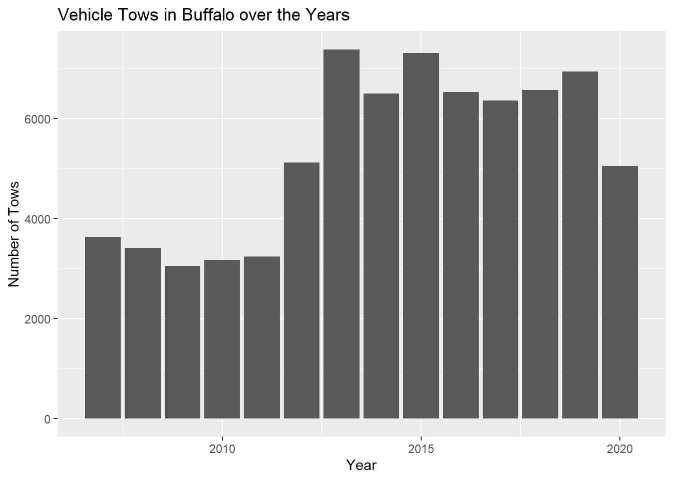
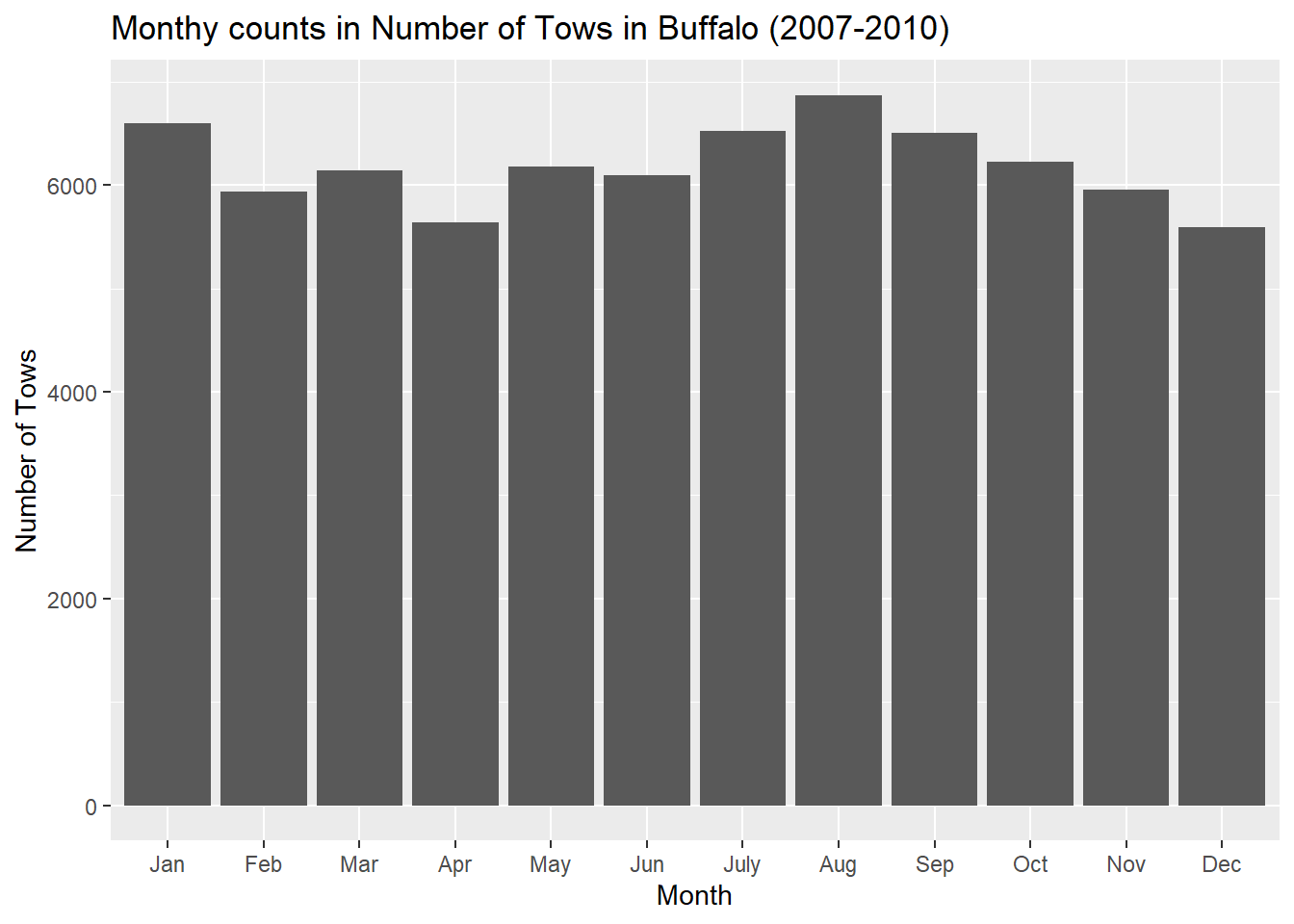
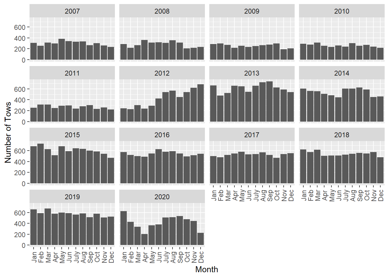
I did my analysis to find out the reasons for towing and variation in towing counts with respect to different month of year (seasonal variation). I also looked at how towing count are changing over the year. Final I made a interactive map with tows clustered in a location if it had several tows occurrences.This map could help us to identify the locations of tows. A lot of tows happen because of accidents. So this map can help us identify the locations of accidents.

Number of Tow in different Police district

We can see from the followings table that Police Districts D and E have the highest number of tows.

POLICE DISTRICT	Number of Tows
District A	9955
District B	14680
District C	15883
District D	16991
District E	16438
NA	332

Reasons for Towing

TOW DESCRIPTION	Number of Tows
ABANDONED VEHICLE	7890
ACCIDENT	13940
FAILURE TO CLAIM	13
GONE ON ARRIVAL	1786
ILLEGAL VEHICLE	33358
ILLEGALLY PARKED	6868
IMPOUNDED	6164
STOLEN VEHICLE	4260

Yearly Towing Counts

Monthly Variation in Tow Counts

Time series Plot of Daily Towing count in Buffalo

dygraph(tow_xts,main="Daily Tow count in Buffalo, NY")%>%
  dyRangeSelector(dateWindow = c("2007-01-01", "2019-03-26"))

Please change range of time in the bottom to get more specific time data

Showing All Tows in interactive Map

new_data <- data %>%
   filter(LONGITUDE!="NA"|LATITUDE!="NA")
all_tow <- leaflet(new_data) %>% 
   addTiles() %>% 
   setView( lng = -78.84, lat = 42.9, zoom = 12 ) %>%
   addProviderTiles("Esri.WorldTopoMap") %>%
   addCircleMarkers(lng = ~LONGITUDE,
                    lat = ~LATITUDE,
                    clusterOptions = markerClusterOptions()) %>%
   setMaxBounds(lng1=-78.7,lat1=42.8,
                lng2=-79,lat2=42.98)
all_tow

Please zoom in/out to see the location of towing

Towing related to DIFFERENT REASONS

AB <- new_data %>%
   filter(`TOW DESCRIPTION`=="ABANDONED VEHICLE")
ACC <- new_data %>%
   filter(`TOW DESCRIPTION`=="ACCIDENT")
FC <- new_data %>%
   filter(`TOW DESCRIPTION`=="FAILURE TO CLAIM")
GA <- new_data %>%
   filter(`TOW DESCRIPTION`=="GONE ON ARRIVAL")
ILLV <- new_data %>%
   filter(`TOW DESCRIPTION`=="ILLEGAL VEHICLE")
ILLP <- new_data %>%
   filter(`TOW DESCRIPTION`=="ILLEGALLY PARKED")
IMP <- new_data %>%
   filter(`TOW DESCRIPTION`=="IMPOUNDED")
STL <- new_data %>%
   filter(`TOW DESCRIPTION`=="STOLEN VEHICLE")
reasons <- leaflet(ACC) %>% 
   addTiles() %>% 
   addProviderTiles("Esri.WorldTopoMap") %>%
   setView( lng = -78.84, lat = 42.9, zoom = 12) %>%
   setMaxBounds(lng1=-78.7,lat1=42.8,
                lng2=-79,lat2=42.98) %>%
   addCircleMarkers(lng = ~LONGITUDE,
                    lat = ~LATITUDE,
                    group="ACCIDENT",
                    clusterOptions = markerClusterOptions()) %>%
   addCircleMarkers(data=AB,
                    lng = ~LONGITUDE,
                    lat = ~LATITUDE,
                    group="ABANDONED VEHICLE",
                    clusterOptions = markerClusterOptions()) %>%
   addCircleMarkers(data=FC,
                    lng = ~LONGITUDE,
                    lat = ~LATITUDE,
                    group="FAILURE TO CLAIM",
                    clusterOptions = markerClusterOptions()) %>%
   addCircleMarkers(data=GA,
                    lng = ~LONGITUDE,
                    lat = ~LATITUDE,
                    group="GONE ON ARRIVAL",
                    clusterOptions = markerClusterOptions()) %>%
   addCircleMarkers(data=ILLV,
                    lng = ~LONGITUDE,
                    lat = ~LATITUDE,
                    group="ILLEGAL VEHICLE",
                    clusterOptions = markerClusterOptions()) %>%
   addCircleMarkers(data=ILLP,
                    lng = ~LONGITUDE,
                    lat = ~LATITUDE,
                    group="ILLEGALLY PARKED",
                    clusterOptions = markerClusterOptions()) %>%
   addCircleMarkers(data=IMP,
                    lng = ~LONGITUDE,
                    lat = ~LATITUDE,
                    group="IMPOUNDED",
                    clusterOptions = markerClusterOptions()) %>%
   addCircleMarkers(data=STL,
                    lng = ~LONGITUDE,
                    lat = ~LATITUDE,
                    group="STOLEN VEHICLE",
                    clusterOptions = markerClusterOptions()) %>%
   
   addLayersControl(overlayGroups = c("ACCIDENT", "ABANDONED VEHICLE","FAILURE TO CLAIM","GONE ON ARRIVAL","ILLEGAL VEHICLE","ILLEGALLY PARKED","IMPOUNDED","STOLEN VEHICLE"))
reasons

Please zoom in/out to see the location of towing related to accident. Also look at the top right corners to see locations for different reasons.

Conclusions

A lot of the Tows are happening because of the accidents. If we look at the location of the tows related to accidents we can see that the accidents are occuring mostly at the intersection.Also the number of tows are increasing over the year.We can see from the table that police district D and E have the most number of tows. For seasonal variation we can look at the histogram of tows with respect to the months.We can see from the histogram that january has a lot of tow occurance and then there is a decrease and then another increase in around july to august and then again decreasing gradually. December-january are the start of snow season. That’s why I think there in an increase in the number of tows. Then people might get used to snow and the number of tow decrease. July, august are the time of summer and fall and people usually go out and make more recreational trips around this time which might be the reason for increase in trips.

References

1. https://data.buffalony.gov/Transportation/Tows/5c88-nfii
2. DataCamp course list: https://learn.datacamp.com/courses/interactive-maps-with-leaflet-in-r https://learn.datacamp.com/courses/introduction-to-data-visualization-with-ggplot2 https://learn.datacamp.com/courses/introduction-to-the-tidyverse

This website is a project for Adam Wilson's Spatial Data Science (GEO511) Course at the University at Buffalo