Tick-borne Pathogen Prevalence and Forest Cover in New York State
Collin O’Connor
Introduction
The deer tick or blacklegged tick (Ixodes scapularis) is the most medically relevant species of hard tick found in New York State (NYS). I. scapularis populations in NYS may carry a plethora of pathogens, including but not limited to:
- Borrelia burgdorferi - the agent of Lyme disease (1)
- Anaplasma phagocytophilum - the agent of human granulocytic anaplasmosis (2)
- Babesia microti - the agent of babesiosis in humans (3)
- Borrelia miyamotoi - causative of hard tick relapsing tick fever (4)
The prevalence of the above pathogens varies both spatially and temporally in NYS, which results in varying risk for NYS residents (5). Because these pathogens are not transmitted from tick to tick transovarially, they are required to be maintained throughout populations of animal reservoir hosts in the various ecosystems of NYS. Data suggests that certain land use and land cover types are beneficial for populations of animals which maintain these pathogens (4), and potentially for the pathogen’s themselves (6). This project aims to explore any trends between pathogen prevalence within I. scapularis at the county level and land use / land cover types in NYS.
Materials and methods
Methods - Software information
All data processing and analysis were preformed using RStudio with the following version specifications and packages:
## R version 4.0.2 (2020-06-22)
## Platform: x86_64-apple-darwin17.0 (64-bit)
## Running under: macOS 10.16
##
## Matrix products: default
## BLAS: /Library/Frameworks/R.framework/Versions/4.0/Resources/lib/libRblas.dylib
## LAPACK: /Library/Frameworks/R.framework/Versions/4.0/Resources/lib/libRlapack.dylib
##
## locale:
## [1] en_US.UTF-8/en_US.UTF-8/en_US.UTF-8/C/en_US.UTF-8/en_US.UTF-8
##
## attached base packages:
## [1] stats graphics grDevices utils datasets methods base
##
## other attached packages:
## [1] sjstats_0.18.0 pscl_1.5.5 sjlabelled_1.1.7 sjmisc_2.8.5
## [5] sjPlot_2.8.6 glue_1.4.2 tmap_3.2 rgeos_0.5-5
## [9] rgdal_1.5-18 gdalUtils_2.0.3.2 leaflet_2.0.3 spData_0.3.8
## [13] sf_0.9-6 raster_3.3-13 sp_1.4-4 FedData_3.0.0.9000
## [17] forcats_0.5.0 stringr_1.4.0 dplyr_1.0.2 purrr_0.3.4
## [21] tidyr_1.1.2 tibble_3.0.4 ggplot2_3.3.2 tidyverse_1.3.0
## [25] readr_1.4.0
##
## loaded via a namespace (and not attached):
## [1] minqa_1.2.4 TH.data_1.0-10 leafem_0.1.3
## [4] colorspace_1.4-1 ellipsis_0.3.1 class_7.3-17
## [7] estimability_1.3 parameters_0.9.0 base64enc_0.1-3
## [10] fs_1.5.0 dichromat_2.0-0 rstudioapi_0.11
## [13] mvtnorm_1.1-1 fansi_0.4.1 lubridate_1.7.9
## [16] xml2_1.3.2 splines_4.0.2 codetools_0.2-16
## [19] R.methodsS3_1.8.1 knitr_1.30 jsonlite_1.7.1
## [22] nloptr_1.2.2.2 ggeffects_0.16.0 tmaptools_3.1
## [25] broom_0.7.1 dbplyr_1.4.4 png_0.1-7
## [28] R.oo_1.24.0 effectsize_0.4.0 compiler_4.0.2
## [31] httr_1.4.2 emmeans_1.5.1 backports_1.1.10
## [34] Matrix_1.2-18 assertthat_0.2.1 cli_2.1.0
## [37] leaflet.providers_1.9.0 htmltools_0.5.0 tools_4.0.2
## [40] coda_0.19-4 gtable_0.3.0 Rcpp_1.0.5
## [43] cellranger_1.1.0 vctrs_0.3.4 nlme_3.1-149
## [46] iterators_1.0.13 leafsync_0.1.0 crosstalk_1.1.0.1
## [49] insight_0.10.0 lwgeom_0.2-5 xfun_0.18
## [52] lme4_1.1-23 rvest_0.3.6 lifecycle_0.2.0
## [55] statmod_1.4.34 XML_3.99-0.5 zoo_1.8-8
## [58] MASS_7.3-53 scales_1.1.1 hms_0.5.3
## [61] sandwich_3.0-0 parallel_4.0.2 RColorBrewer_1.1-2
## [64] yaml_2.2.1 stringi_1.5.3 bayestestR_0.7.5
## [67] foreach_1.5.1 spDataLarge_0.4.1 e1071_1.7-4
## [70] boot_1.3-25 rlang_0.4.8 pkgconfig_2.0.3
## [73] evaluate_0.14 lattice_0.20-41 htmlwidgets_1.5.2
## [76] tidyselect_1.1.0 magrittr_1.5 R6_2.5.0
## [79] generics_0.1.0 multcomp_1.4-14 DBI_1.1.0
## [82] pillar_1.4.6 haven_2.3.1 withr_2.3.0
## [85] units_0.6-7 stars_0.4-3 survival_3.2-7
## [88] abind_1.4-5 performance_0.5.1 modelr_0.1.8
## [91] crayon_1.3.4 KernSmooth_2.23-17 rmarkdown_2.4
## [94] grid_4.0.2 readxl_1.3.1 data.table_1.13.2
## [97] blob_1.2.1 reprex_0.3.0 digest_0.6.27
## [100] classInt_0.4-3 xtable_1.8-4 R.utils_2.10.1
## [103] munsell_0.5.0 viridisLite_0.3.0Methods - Data Gathering
The data for this project are gathered from three main sources. The first source is the New York State Department of Health (NYSDOH) Vector Ecology Laboratory’s tick borne pathogen surveillance dataset. This dataset contains host-seeking tick field surveillance data throughout NYS from 2008 - present, as well as corresponding molecular testing data for the four pathogens mentioned in the introduction. These data are spatially aggregated to the county level and are available online at the following links for Nymphs and Adults: These data were gathered into R using the following code:
tdir=tempdir()
adulturl <- "https://health.data.ny.gov/api/views/vzbp-i2d4/rows.csv?accessType=DOWNLOAD&bom=true&query=select+*"
nymphurl <- "https://health.data.ny.gov/api/views/kibp-u2ip/rows.csv?accessType=DOWNLOAD&bom=true&query=select+*"
if(file.exists(paste(tdir,"/Adultdata.csv",sep=""))==FALSE){
download.file(adulturl, destfile = file.path(tdir,"/Adultdata.csv"))}
if(file.exists(paste(tdir,"/Nymphdata.csv",sep=""))==FALSE){
download.file(nymphurl,destfile = file.path(tdir,"/Nymphdata.csv"))}
Nymphdata <- read_csv(paste(tdir,"/Nymphdata.csv",sep=""))
Adultdata <- read_csv(paste(tdir,"/Adultdata.csv",sep=""))These data were cleaned using the code shown in this hidden code chunk. The code to preform this data cleaning is not elegant and thus was hidden to save space. Feel free to view if necessary.
names(Adultdata)[6]="Total_Tested"
Adult_BBdat=Adultdata[,1:7]
Adult_BBdat$Pathogen="Borrelia burgdorferi"
names(Adult_BBdat)[7]="Percent_Positive"
Adult_Apdat=Adultdata[,c(1:6,8)]
Adult_Apdat$Pathogen="Anaplasma phagocytophilum"
names(Adult_Apdat)[7]="Percent_Positive"
Adult_Bmiydat=Adultdata[,c(1:6,10)]
Adult_Bmiydat$Pathogen="Borrelia miyamotoi"
names(Adult_Bmiydat)[7]="Percent_Positive"
Adult_Bmicdat=Adultdata[,c(1:6,9)]
Adult_Bmicdat$Pathogen="Babesia microti"
names(Adult_Bmicdat)[7]="Percent_Positive"
Adultnewdat1 = rbind(Adult_BBdat,Adult_Apdat)
Adultnewdat1 = rbind(Adultnewdat1,Adult_Bmiydat)
Adultnewdat1 = rbind(Adultnewdat1,Adult_Bmicdat)
Adultnewdat1$`Percent Positiveby100`=Adultnewdat1$`Percent_Positive`/100
Adultnewdat1$Totpos=round(Adultnewdat1$`Total_Tested`*Adultnewdat1$`Percent Positiveby100`)
Adultnewdat2 = subset(Adultnewdat1,is.na(Adultnewdat1$Percent_Positive)==FALSE)
Adulttotpos = Adultnewdat2 %>%
group_by(Year,Pathogen) %>%
summarize(sum(Totpos))
Adulttotpos$`sum(Totpos)` = ifelse(is.na(Adulttotpos$`sum(Totpos)`)==TRUE,0,Adulttotpos$`sum(Totpos)`)
Adulttottested = Adultnewdat2 %>%
group_by(Year,Pathogen) %>%
summarize(sum(Total_Tested))
Adultgroupings=cbind(Adulttottested,Adulttotpos)
Adultgroupings=Adultgroupings[,c(1:3,6)]
Adultgroupings$percpos=(Adultgroupings$`sum(Totpos)`/Adultgroupings$`sum(Total_Tested)`)*100
names(Adultgroupings)[1]="Year"
names(Adultgroupings)[2]="Pathogen"
Adultgroupings$`Life Stage`="Adult"
names(Nymphdata)[6]="Total_Tested"
Nymph_BBdat=Nymphdata[,1:7]
Nymph_BBdat$Pathogen="Borrelia burgdorferi"
names(Nymph_BBdat)[7]="Percent_Positive"
Nymph_Apdat=Nymphdata[,c(1:6,8)]
Nymph_Apdat$Pathogen="Anaplasma phagocytophilum"
names(Nymph_Apdat)[7]="Percent_Positive"
Nymph_Bmiydat=Nymphdata[,c(1:6,10)]
Nymph_Bmiydat$Pathogen="Borrelia miyamotoi"
names(Nymph_Bmiydat)[7]="Percent_Positive"
Nymph_Bmicdat=Nymphdata[,c(1:6,9)]
Nymph_Bmicdat$Pathogen="Babesia microti"
names(Nymph_Bmicdat)[7]="Percent_Positive"
Nymphnewdat1 = rbind(Nymph_BBdat,Nymph_Apdat)
Nymphnewdat1 = rbind(Nymphnewdat1,Nymph_Bmiydat)
Nymphnewdat1 = rbind(Nymphnewdat1,Nymph_Bmicdat)
Nymphnewdat1$`Percent Positiveby100`=Nymphnewdat1$`Percent_Positive`/100
Nymphnewdat1$Totpos=round(Nymphnewdat1$`Total_Tested`*Nymphnewdat1$`Percent Positiveby100`)
Nymphnewdat2 = subset(Nymphnewdat1,is.na(Nymphnewdat1$Percent_Positive)==FALSE)
Nymphtotpos = Nymphnewdat2 %>%
group_by(Year,Pathogen) %>%
summarize(sum(Totpos))
Nymphtotpos$`sum(Totpos)` = ifelse(is.na(Nymphtotpos$`sum(Totpos)`)==TRUE,0,Nymphtotpos$`sum(Totpos)`)
Nymphtottested = Nymphnewdat2 %>%
group_by(Year,Pathogen) %>%
summarize(sum(Total_Tested))
Nymphgroupings=cbind(Nymphtottested,Nymphtotpos)
Nymphgroupings=Nymphgroupings[,c(1:3,6)]
Nymphgroupings$percpos=(Nymphgroupings$`sum(Totpos)`/Nymphgroupings$`sum(Total_Tested)`)*100
names(Nymphgroupings)[1]="Year"
names(Nymphgroupings)[2]="Pathogen"
Nymphgroupings$`Life Stage`="Nymph"
All_groupings=rbind(Adultgroupings,Nymphgroupings)The second data source is county-level shapefiles from NYS GIS clearinghouse, available at the following link: NYS GIS Clearinghouse. These data were read into R using the following code:
shpurl="http://gis.ny.gov/gisdata/fileserver/?DSID=927&file=NYS_Civil_Boundaries.shp.zip"
if(file.exists(paste(tdir,"/NYS_Civil_Boundaries_SHP/Counties_Shoreline.shp",sep=""))==FALSE){
download.file(shpurl, destfile = file.path(tdir,"Boundaries.zip"))
unzip(file.path(tdir,"Boundaries.zip"),exdir = tdir)}
Cnt=read_sf(paste(tdir,"/NYS_Civil_Boundaries_SHP/Counties_Shoreline.shp",sep=""))
County_Boundaries = Cnt[,c(1,18)]
NYS = st_union(County_Boundaries)
simpSpNYS=st_simplify(NYS,dTolerance=100)
SpNYS=as(NYS,Class="Spatial")Further data cleaning in this code, view if necessary:
Ad_county_totpos = Adultnewdat1 %>%
group_by(Year,Pathogen,County) %>%
summarize(sum(Totpos))
Ad_county_tottested = Adultnewdat1 %>%
group_by(Year,Pathogen,County) %>%
summarize(sum(Total_Tested))
Ad_county_groupings=cbind(Ad_county_tottested,Ad_county_totpos)
Ad_county_groupings=Ad_county_groupings[,c(1:4,8)]
Ad_county_groupings$percpos=Ad_county_groupings$`sum(Totpos)`/(Ad_county_groupings$`sum(Total_Tested)`)*100
names(Ad_county_groupings)=c("Year","Pathogen","County","sum(Total_Tested)","sum(Totpos)","percpos")
Ad_county_groupings$`Life Stage`="Adult"
Ny_county_totpos = Nymphnewdat1 %>%
group_by(Year,Pathogen,County) %>%
summarize(sum(Totpos))
Ny_county_tottested = Nymphnewdat1 %>%
group_by(Year,Pathogen,County) %>%
summarize(sum(Total_Tested))
Ny_county_groupings=cbind(Ny_county_tottested,Ny_county_totpos)
Ny_county_groupings=Ny_county_groupings[,c(1:4,8)]
Ny_county_groupings$percpos=Ny_county_groupings$`sum(Totpos)`/(Ny_county_groupings$`sum(Total_Tested)`)*100
names(Ny_county_groupings)=c("Year","Pathogen","County","sum(Total_Tested)","sum(Totpos)","percpos")
Ny_county_groupings$`Life Stage`="Nymph"
All_county_groupings=rbind(Ad_county_groupings,Ny_county_groupings)
All_county_groupings = subset(All_county_groupings,All_county_groupings$`sum(Total_Tested)`>0)
All_county_groupings = subset(All_county_groupings,is.na(All_county_groupings$`sum(Totpos)`)==FALSE)
Allcnts=as.data.frame(list(unique(All_county_groupings$County)))
names(Allcnts)[1]="County"
Allcnts$ID=c(1:length(unique(All_county_groupings$County)))
All_county_groupings=left_join(All_county_groupings,Allcnts)
All_county_groupings=All_county_groupings[c(-8)]
test_copy=All_groupings
test_copy=test_copy[-c(3,4)]
names(test_copy)[3]="Avg_pos"
test_copy$Pathogen=ifelse(test_copy$Pathogen=="Anaplasma phagocytophilum","A. phagocytophilum",
ifelse(test_copy$Pathogen=="Babesia microti","B. microti",
ifelse(test_copy$Pathogen=="Borrelia burgdorferi","B. burgdorferi",
ifelse(test_copy$Pathogen=="Borrelia miyamotoi","B. miyamotoi",NA))))
test_copy$Pathogen1=ifelse(test_copy$Pathogen=="A. phagocytophilum","NYS Average A. phagocytophilum",
ifelse(test_copy$Pathogen=="B. microti","NYS Average B. microti",
ifelse(test_copy$Pathogen=="B. burgdorferi","NYS Average B. burgdorferi",
ifelse(test_copy$Pathogen=="B. miyamotoi","NYS Average B. miyamotoi",NA))))
All_county_groupings$Pathogen=ifelse(All_county_groupings$Pathogen=="Anaplasma phagocytophilum","A. phagocytophilum",
ifelse(All_county_groupings$Pathogen=="Babesia microti","B. microti",
ifelse(All_county_groupings$Pathogen=="Borrelia burgdorferi","B. burgdorferi",
ifelse(All_county_groupings$Pathogen=="Borrelia miyamotoi","B. miyamotoi",NA))))
asdf=as.data.frame(c(2008:2019))
names(County_Boundaries)[1]="County"
names(asdf)[1]="Year"
asdf$County= c(subset(County_Boundaries$County, !(County_Boundaries$County %in% All_county_groupings$County)),
subset(County_Boundaries$County, !(County_Boundaries$County %in% All_county_groupings$County)))
asdf$Pathogen=c("A. phagocytophilum","B. microti","B. miyamotoi","B. burgdorferi","A. phagocytophilum",
"B. microti","B. miyamotoi","B. burgdorferi","A. phagocytophilum","B. microti","B. miyamotoi","B. burgdorferi")
asdf$Life_Stage=c("Nymph","Nymph","Nymph","Nymph","Nymph","Nymph",
"Adult","Adult","Adult","Adult","Adult","Adult")
asdf2=tidyr::expand(asdf,Year,County,Pathogen,Life_Stage)
asdf2$Total_tested=0
asdf2$Tot_pos=0
asdf2$percpos=0
names(All_county_groupings)[4]="Total_tested"
names(All_county_groupings)[5]="Tot_pos"
names(All_county_groupings)[7]="Life_Stage"
All_county_groupings2=rbind(All_county_groupings,asdf2)
All_county_groupings3=tidyr::expand(All_county_groupings2,Year,Pathogen,County,Life_Stage)
All_county_groupings4=left_join(All_county_groupings3,All_county_groupings,by=c("Year","Pathogen","Life_Stage","County"))
names(test_copy)[4]="Life_Stage"The third and final data source is land use and land cover data from the 2016 National Land Cover Dataset, available at the following link: NLCD. These data were downloaded using R-specific NLCD calls. The call was looped to iterate the data download for each county, which would then overwrite the previous county’s data to conserve storage. The analysis was also grouped into this code, which will be explained later.
newcounties=County_Boundaries %>% filter(County != "New York",
County != "Queens",
County != "Kings",
County != "Richmond",
County != "Bronx")
st_transform(newcounties,crs="+proj=utm +zone=18 +datum=NAD83 +units=m +no_defs")
df1=NULL
for(i in 1:nrow(newcounties)){
NLCD=get_nlcd(template = st_as_sf(newcounties[i,]),
year = 2016,
label="Same",
dataset='Land_Cover',
landmass="L48",
extraction.dir = tdir,
force.redo = T)
NLCD2=projectRaster(from=NLCD,crs="+proj=utm +zone=18 +datum=NAD83 +units=m +no_defs")
cropnew=crop(NLCD2,extent(newcounties[i,]))
masknew=mask(cropnew,newcounties[i,])
masknew2= masknew %in% c(41,43)
masknew3=masknew/masknew
df=data.frame(County=paste(newcounties[[i,1]]),
Total_Pixels=cellStats(masknew3,'sum'),
Total_Forest_Pixels=cellStats(masknew2,stat='sum'),
Percent_Forest_Cover=cellStats(masknew2,stat='sum')/cellStats(masknew3,'sum'))
if(is.null(df1)==TRUE){df1=df}
else(df1=rbind(df1,df))}Methods - Data visualization
In order to visualize pathogen prevalence throughout NYS, the ggplot and leaflet packages were used to create time-series graphs and interactive maps. The code to create the NYS average pathogen prevalence time-series graph is shown below:
plot1=ggplot(data = All_groupings,aes(x=Year,y=percpos,color=Pathogen)) +
geom_line() +
ggtitle(expression(paste("Time Series Graph of ",
italic("Ixodes scapularis"),
" Infectivity Rates (NYS)",sep=""))) +
theme(axis.text.x = element_text(angle=65,vjust=.65)) +
geom_hline(yintercept = 0,linetype='solid',color='black',size=.5,alpha=.7) +
geom_vline(xintercept = 2008,linetype='solid',color='black',size=.5,alpha=.7) +
facet_wrap(~`Life Stage`) +
ylab("Pathogen Prevalence (%)")+
scale_x_continuous(breaks=c(2008:2019))The code to create an interactive map where each clicking each county displays a time-series graph comparing county-level pathogen rates to the NYS average is shown below:
test1 = All_county_groupings4 %>%
nest(-County)
dodge=position_dodge(.4)
test2 = test1 %>%
mutate(plot = map2(data, County,
~ggplot()+
geom_hline(yintercept = 0,linetype='solid',color='black',size=.5,alpha=.7)+
geom_vline(xintercept = 2008,linetype='solid',color='black',size=.5,alpha=.7)+
geom_line(data=.x,aes(x=Year,y=percpos,color=Pathogen),position=dodge)+
geom_point(data=.x,aes(x=Year,y=percpos,color=Pathogen),
position=dodge,size=.85)+
scale_color_manual(name="Pathogen",
values=c("#E41A1C","#377EB8","#4DAF4A",
"#984EA3","#E41A1C","#377EB8",
"#4DAF4A","#984EA3"))+
geom_line(data=test_copy,
aes(x=Year,y=Avg_pos,
color=Pathogen,
linetype="NYS Average Pathogen Prevalence"),
position=dodge,)+
scale_linetype_manual("",values = c(2,2,2,2,1,1,1,1))+
theme(axis.text.x = element_text(angle=65,vjust=.65))+
facet_wrap(~Life_Stage)+
scale_x_continuous(breaks=c(2008:2019))+
ylab("Pathogen Prevalence (%)")+
labs(caption="Solid lines indicate pathogen prevalence from sample specimens in County")+
ggtitle(glue("{.y}"))))
County_Boundaries=st_transform(County_Boundaries,CRS("+proj=longlat +datum=WGS84"))
names(County_Boundaries)[1]="County"
test_new=left_join(County_Boundaries,test2,by='County')
plot2=leaflet() %>%
addTiles() %>%
addPolygons(data=test_new,
group='County',
weight=1,
label=~County,
highlight=highlightOptions(
weight=5,
color='red',
bringToFront=TRUE)) %>%
leafpop::addPopupGraphs(graph=test_new$plot,
group='County',
width=600,height=300)Methods - Raster Analysis
NLCD Raster data were used to determine the percent of deciduous and mixed (deciduous/coniferous) forest that covered each county. The code to calculate this data was shown earlier, but a detailed explanation (which ignores the loop) is shown below.
Data for each county is downloaded via this code:
NLCD=get_nlcd(template = st_as_sf(newcounties[i,]),
year = 2016,
label="Same",
dataset='Land_Cover',
landmass="L48",
extraction.dir = tdir,
force.redo = T)The downloaded raster is then projected on to WGS84:
NLCD2=projectRaster(from=NLCD,crs='+proj=longlat +datum=WGS84')The projected raster is then cropped to the extent of the county required:
cropnew=crop(NLCD2,extent(newcounties[i,]))The cropped raster is then masked by the county required:
masknew=mask(cropnew,newcounties[i,])The masked raster is then filtered to only include either deciduous or mixed forest pixels:
masknew2= masknew %in% c(41,43)All pixel values of the original masked raster are then changed to a value of 1, in order to calculate the total number of pixels in the raster:
masknew3=masknew/masknewA dataframe is then compiled which includes the name of the County, the total number of pixels within that county, the total number of mixed/deciduous forest pixels within the county, and the percent of pixels which are mixed/deciduous.
df=data.frame(County=paste(newcounties[[i,1]]),
Total_Pixels=cellStats(masknew3,'sum'),
Total_Forest_Pixels=cellStats(masknew2,stat='sum'),
Percent_Forest_Cover=cellStats(masknew2,stat='sum')/cellStats(masknew3,'sum'))Methods - Statistical Analysis
Following the collection of pathogen and raster data, each variable was examined for normality. The distribution of each variable determined the type of analysis used. For analysis, pathogen prevalence was always the dependent variable. If both the percent forest cover and pathogen prevalence variables were normal, a simple test for correlation was used. If the pathogen prevalence variable seemed to follow a negative binomial distribution, the zero-inflated negative binomial regression model was used.
Results
Results - NYS Average Rates Within I. scapularis Populations
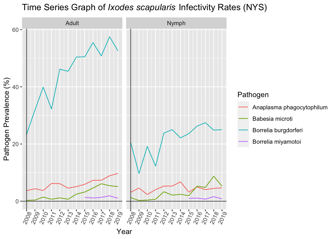
Pathogen prevalence in NYS shows a general trend of increase over time. Average rates of each pathogen are consistent with expectations where B. burgdorferi shows the highest prevalence within I. scapularis populations in NYS. A. phagocytophilum , B. microti , and B. miyamotoi exhibit the second, third, and fourth highest prevalence, respectively. Additionally, prevalence of each pathogen is about half as much in nymphal ticks compared to adult ticks.
Results - County Average Rates Within I. scapularis Populations
General takeaways from the interactive county level map are the following:
- Rates in the capital district and metropolitan areas of NYS are generally higher than the NYS average, and also have more complete data.
- The north county (Adirondack region) has generally low prevalence numbers (likely due to low numbers of tick populations).
- In counties with complete data, pathogen prevalence generally has risen over time.
Results - Forest Cover by County in New York State
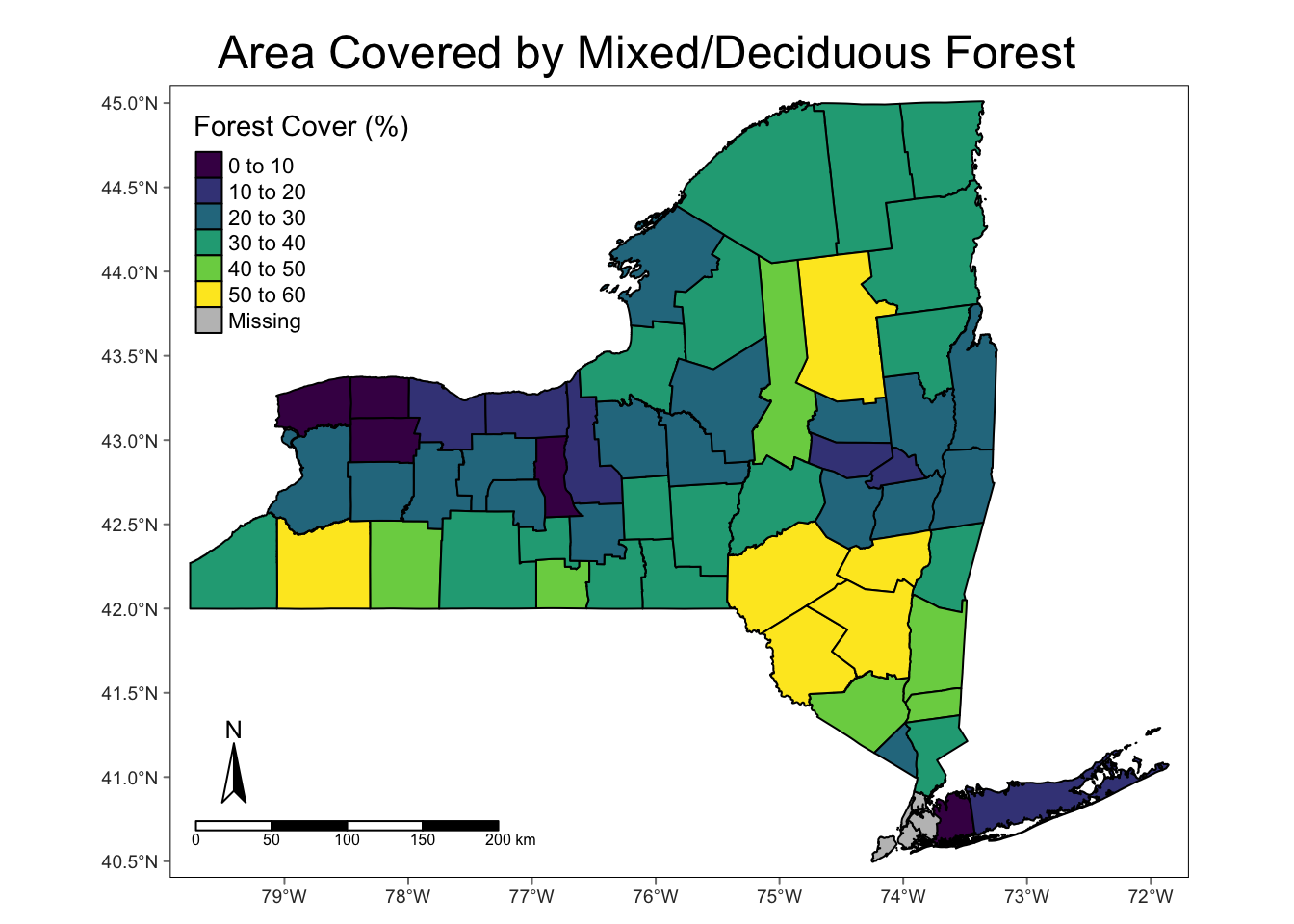
The main takeaway from the above map is that the counties with the highest percentage of forest cover are those counties in the Adirondack and Catskill mountain regions. This is important to note, because these areas are at higher elevation, which is generally poorer habitat for I. scapularis , resulting in lower density. This phenomenon has the potential to alter the results of pathogen prevalence, which will be shown later.
Results - Statistical Analysis
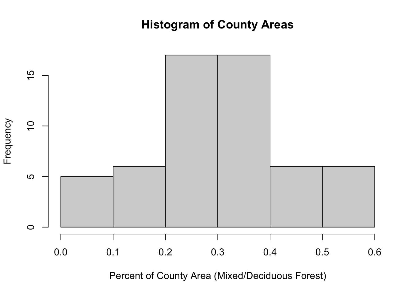
The percent area of each county covered by deciduous or mixed forest appears normally distributed.
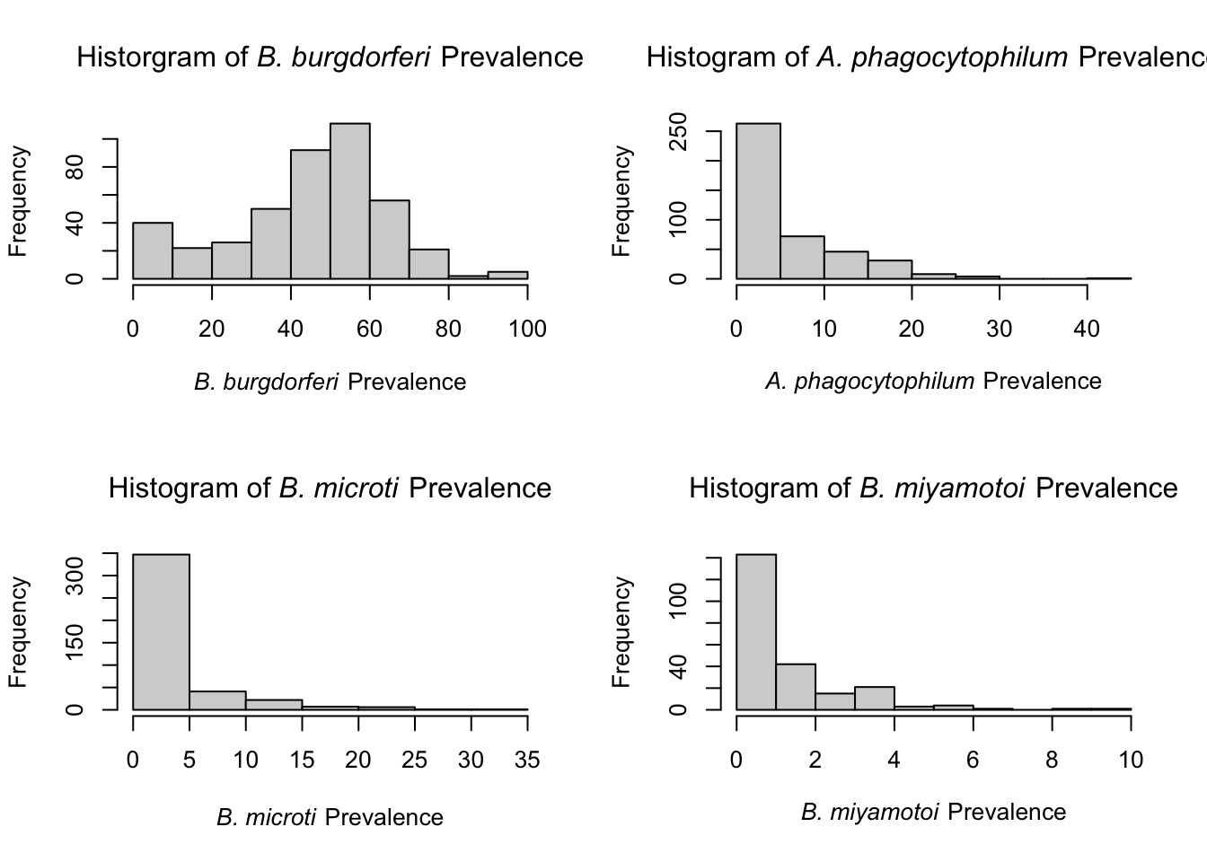
B. burgdorferi appears to be the only normally distributed pathogen data among adult ticks. This likely occurs because it has the highest pathogen prevalence and is endemic throughout NYS. Prevalence among all other pathogens appears to be zero-inflated, likely because the number of positives are low. Lower numbers make the pathogen data approach a Poisson/negative binomial distribution because it is count data.
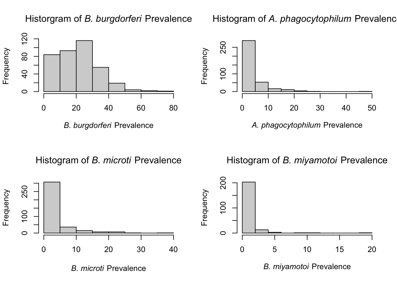
Similar to adults ticks, B. burgdorferi prevalence among nymphs is near a normal distribution. All others approach Poisson/negative binomial distribution. Due to the normality of B. burgdorferi , Pearson correlation tests were used to examine the relationship between percent mixed/deciduous forest cover and B. burgdorferi prevalence.
Adult test is shown below:
##
## Pearson's product-moment correlation
##
## data: adulttestingdata$Percent_Forest_Cover and adulttestingdata$`B. burgdorferi (%)`
## t = -0.24767, df = 423, p-value = 0.8045
## alternative hypothesis: true correlation is not equal to 0
## 95 percent confidence interval:
## -0.10703993 0.08317493
## sample estimates:
## cor
## -0.01204144The p-value from the test of correlation between county-level percent forest cover and adult B. burgdorferi prevalence fails to reject the null hypothesis, indicating there is no correlation in this sample.
Nymph test is shown below:
##
## Pearson's product-moment correlation
##
## data: nymphtestingdata$Percent_Forest_Cover and nymphtestingdata$`B. burgdorferi (%)`
## t = 0.32964, df = 372, p-value = 0.7419
## alternative hypothesis: true correlation is not equal to 0
## 95 percent confidence interval:
## -0.08446414 0.11829025
## sample estimates:
## cor
## 0.01708873Similar to adults, the p-value from the test of correlation between county-level percent forest cover and nymphal B. burgdorferi prevalence fails to reject the null hypothesis, indicating there is no correlation in this sample.
To examine the relationship between percent mixed/deciduous forest cover and A. phagocytophilum B. microti , and B. miyamotoi prevalence, zero-inflated negative binomial (ZINB) models were used. The dependent variable for each count and zero-inflated model was the count of samples testing positive for a particular pathogen, where the independent variable was percent mixed/deciduous forest cover. Code to create each model for both adults and nymphs is shown below:
adult_ANA_reg=zeroinfl(formula = ANApos ~ Percent_Forest_Cover | Percent_Forest_Cover,
data=adulttestingdata,dist='negbin')
adult_Bmic_reg=zeroinfl(formula = Bmicpos ~ Percent_Forest_Cover | Percent_Forest_Cover,
data=adulttestingdata,dist='negbin')
adult_Bmiya_reg=zeroinfl(formula = Bmiyapos ~ Percent_Forest_Cover | Percent_Forest_Cover,
data=adulttestingdata,dist='negbin')nymph_ANA_reg=zeroinfl(formula = ANApos ~ Percent_Forest_Cover | Percent_Forest_Cover,
data=nymphtestingdata,dist='negbin')
nymph_Bmic_reg=zeroinfl(formula = Bmicpos ~ Percent_Forest_Cover | Percent_Forest_Cover,
data=nymphtestingdata,dist='negbin')
nymph_Bmiya_reg=zeroinfl(formula = Bmiyapos ~ Percent_Forest_Cover | Percent_Forest_Cover,
data=nymphtestingdata,dist='negbin')| A. phagocytophilum | B. microti | B. miyamotoi | |
|---|---|---|---|
| Predictors | p | p | p |
| (Intercept) | <0.001 | <0.001 | 0.001 |
| Percent_Forest_Cover | 0.266 | 0.135 | 0.005 |
| Zero-Inflated Model | |||
| (Intercept) | 0.093 | 0.165 | 0.225 |
| Percent_Forest_Cover | 0.055 | 0.141 | 0.139 |
| Observations | 425 | 425 | 231 |
Coefficient of adult B. miyamotoi model shown below:
adult_Bmiya_reg$coefficients$count## (Intercept) Percent_Forest_Cover
## 0.9398944 -2.3622950| A. phagocytophilum | B. microti | B. miyamotoi | |
|---|---|---|---|
| Predictors | p | p | p |
| (Intercept) | <0.001 | <0.001 | 0.141 |
| Percent_Forest_Cover | 0.183 | <0.001 | 0.002 |
| Zero-Inflated Model | |||
| (Intercept) | 0.052 | 0.183 | NaN |
| Percent_Forest_Cover | 0.024 | 0.188 | NaN |
| Observations | 374 | 374 | 222 |
Coefficient of statistically significant nymphal models shown below:
Nymphal A. phagocyotphilum zero-inflated model:
nymph_ANA_reg$coefficients$zero## (Intercept) Percent_Forest_Cover
## 5.398699 -73.873538Nymphal B. microti count model:
nymph_Bmic_reg$coefficients$count## (Intercept) Percent_Forest_Cover
## 1.986349 -3.640456Nymphal B. miyamotoi count model:
nymph_Bmiya_reg$coefficients$count## (Intercept) Percent_Forest_Cover
## 0.510452 -3.406799Conclusions
Tick-borne pathogen prevalence in NYS is an ever-increasing problem. NYSDOH Vector Ecology Laboratory tick sampling indicates that pathogen prevalence of B. burgdorferi , A. phagocytophilum , B. microti , and B. miyamotoi in host-seeking ticks have been increasing over time. Increases in pathogen prevalence provides a warning for increased risk of tick-borne disease for NYS citizens. Although the prevalence of each pathogen, and thus, risk for disease differs by county, the general trend indicates that tick-borne disease will be an issue for years to come in NYS. The interactive map in this project provides a user-friendly interface to navigate publicly available data and to determine the potential risk for tick-borne pathogen exposure in your county.
One extremely important factor in determining risk for tick-borne pathogen exposure is tick habitat.< I. scapularis prefer deciduous and mixed forest ecosystems, making tick prevention methods in these ecosystems an important topic for reducing tick-borne disease risk in the future. This analysis aimed to determine if the percent of a county covered by these types of forest plays any role in pathogen prevalence rates. The method behind this thinking is that the more available area for tick populations to expand dually provides tick-borne pathogens the ability to expand into these areas. Coincidentally, preliminary results from the correlation tests and ZINB modeling show that the percent of a county covered by mixed or deciduous forest is either not directly related to tick-borne pathogen prevalence, or actually shows a decreased risk for pathogen prevalence. There are a few likely explanations for these results. The first is that aggregating forest cover to large spatial areas (counties in this study), do not represent the microvariations in tick habitat that allow populations to proliferate. Smaller spatial scales may provide a more accurate representation of the relationship between land cover and pathogen prevalence. A possible cause of the mixed results in this study are due to the counties with the highest forest cover being at higher elevations. I. scapularis density generally decreases as elevation increases, likely due to host species ranges. This can cause some confounding between forest cover and elevation, confusing the effect of each variable on tick density. A final explanation is that there is sampling bias in these data. The NYSDOH is tasked with protecting the health of the public, and thus, sampling is generally conducted:
- Where the greatest risk for tick-human interaction is.
- Where the density of tick populations is high enough to obtain sufficient sample size.
The first bias would cause more data to be gathered around suburban areas due to the larger number of individuals at risk. Counties with more suburban areas will likely have a lower percentage of forest cover, thus biasing the data.
The second bias would cause more data to be gathered in areas where tick populations are large enough for the purpose of sampling. Often times, this occurs in areas with forest edge and nearby woodlots. These types of areas represent microecosystems perfect for tick population expansion, thus, making sampling easier for NYSDOH staff.
In summation, the two takeaways from this project are the following:
- Tick pathogen prevalence has been increasing over time in NYS.
- Tick pathogen prevalence varies spatially throughout NYS.
- A more detailed analysis is required to examine the role forest cover plays with pathogen prevalence.
References
1.) Chen H, White DJ, Caraco TB, Stratton HH. Epidemic and Spatial Dynamics of Lyme Disease in New York State, 1990–2000. J Med Entomol. 2005;42(5):10.
2.) Chen S-M, Dumler JS, Bakken JS, Walker DH. Identificatin of a Granulocytotropic Ehrlichia Species as the Etiologic Agent of Human Disease. J Clin Microbiol. 1994;32(3):589-595.
3.) Spielman A, Wilson ML, Levine JF, Piesman J. Ecology of Ixodes Dammini-Borne Human Babesiosis and Lyme Disease. Annu Rev Entomol. 1985;30(1):439-460. doi:10.1146/annurev.en.30.010185.002255
4.) Piedmonte N, Shaw SB, Prusinski M, Fierke MK. Landscape Features Associated With Blacklegged Tick (Acari: Ixodidae) Density and Tick-Borne Pathogen Prevalence at Multiple Spatial Scales in Central New York State. J Med Entomol. 2018;55(6):1496-1508. doi:10.1093/jme/tjy111
5.) Joseph JT, John M, Visintainer P, Wormser GP. Increasing incidence and changing epidemiology of babesiosis in the Hudson Valley region of New York State: 2009-2016. Diagn Microbiol Infect Dis. 2020;96:1-3.
6.) Prusinski MA, Chen H, Drobnack JM, et al. Habitat Structure Associated with Borrelia burgdorferi Prevalence in Small Mammals in New York State. Environ Entomol. 2006;35(2):308-319.