Reported Domestic Violence in Chicago City, IL
Before and After the COVID-19 Lockdown
Ting Chang
1 Introduction
The surging cases of COVID-19 in spring 2020 has caused governments around the world to impose lock-down policy (stay home order) in order to slow down the spread of pandemic. While COVID-19 is a worldwide health crisis, some researchers (Ertan et al., (2020); Bradbury‐Jones and Isham, (2020)) have expressed concerns for another crucial public health threat, domestic violence, which is expected to increase while more people were constrained at home.
This project aims to explore the spatial and temporal distribution of the domestic violence in Chicago City, Illinois using the crime reported data. In particularly, to examine whether the reported domestic violence has increased as expected after the authorities have imposed lock-down policy.
2 Materials and methods
2.1 Set Up
In order to run the code below, firstly, we need to load the following packages in R, you might need to install some of them in ahead. If your environment and locale is not set to English, utilizing the two lines start with Sys., it would help plotting the date label in English. Otherwise, please comment out these two lines.
library(tidyverse)
library(tidycensus)
library(kableExtra)
library(ggplot2)
library(sf)
library(RColorBrewer)
library(viridis)
library(gridExtra)
library(classInt)

knitr::opts_chunk$set(cache=TRUE)  # cache the results for quick compiling

# For plotting date label in English
Sys.setenv("LANGUAGE"="En")
Sys.setlocale("LC_ALL", "English")

# Changing environment and locale language learned from:
# https://stackoverflow.com/questions/15438429/axis-labels-are-not-plotted-in-english
2.2 Data Import and Processing
In this part, our goal is to prepare the data for the analysis below. We want to obtain the following data:
- The basic geographic unit for the analysis:
- census block group spatial data
- The primary variable for our analysis:
- Domestic violence count
- Domestic violence rate
- Domestic violence count
- The social-economics factors for the domestic violence:
- Crime rate
- Median household income
- Unemployment rate
- Crime rate
And we will obtain these datasets from the following data source:
- Census TIGER data (Data has already been processed and provided in the data folder.)
- Census data - American Community Survey 5-year estimated (2018)
- Crime reported data from Chicago Data Portal
2.2.1 Chicago City’s census block group shapefile
Load the data
The Chicago City’s census block group shapefile is provided in the data folder. I have obtained it previously from the census TIGER data.
# Load chicago CBG shapefile in R
chicago_cbg <- st_read("data/chicago_cbg.shp") %>%
  select(CensusBloc)
2.2.2 Census data
Data download
We will download several datasets from the American Community Survey 5-Year data at the census block group level using the lovely package, tidycensus. Since the newest released estimated data is the 2018 year version, we will download data from 2018.
# For searching variables from ACS-5yr 2018
v18 <- load_variables(2018, "acs5", cache = TRUE)

# Downloading population data
population_18 <- get_acs(geography = "block group",
                         variables = c(population = "B01003_001"),
                         state = "IL",
                         county = c("Cook", "DuPage"),
                         year = 2018)

# Downloading median household income data
median_income_18 <- get_acs(geography = "block group",
                            variables = c(medincome = "B19013_001"),
                            state = "IL",
                            county = c("Cook", "DuPage"),
                            year = 2018)

# Downloading employment data
employment_18 <- get_acs(geography = "block group",
                         variables = c(total_in_labor = "B23025_002", unemployed = "B23025_005"),
                         state = "IL",
                         county = c("Cook", "DuPage"),
                         year = 2018,
                         output = "wide")
Data Processing
Afterwards, we will crop the obtained census data to the Chicago City using the pre-loaded shapefile and slightly tidy up our data.
# Population data
population_18 <- left_join(chicago_cbg, population_18, by = c("CensusBloc" = "GEOID")) %>%
  select(CensusBloc, population = estimate)

# Median household income data
median_income_18 <- left_join(chicago_cbg, median_income_18, by = c("CensusBloc" = "GEOID")) %>%
  select(CensusBloc, median_income = estimate)

# Unemployment rate data
employment_18 <- left_join(chicago_cbg, employment_18, by = c("CensusBloc" = "GEOID")) %>%
  # calculate the unemployment rate by dividing the unemployed population by the total in labor population
  select(CensusBloc, total_in_labor = total_in_laborE, unemployed = unemployedE) %>%
  mutate(unemployment_rate = unemployed/total_in_labor)
2.2.3 Crime reported data
Data download
The crime reported data will be obtained from the Chicago Data Portal via Socrata Open Data API. If the API does not work, try download the .csv file from the provided link.
# Download crime reported data and load it in R
dataurl = "https://data.cityofchicago.org/resource/ijzp-q8t2.csv?$order=Date DESC&$limit=460000&$offset=20000"
tdir = tempdir()
download.file(dataurl, destfile = file.path(tdir, "chicago_crime.csv"))

chicago_crime <- read_csv(paste(tdir,"/chicago_crime.csv", sep = ""))

# Tidy the data
chicago_crime_clean <- chicago_crime %>%
  mutate(date = as.Date(date, "%Y.%m.%d")) %>%
  filter(as.Date(date) >= "2018-12-31" & as.Date(date) <= "2020-10-04") %>%
  select(-block, -iucr, -beat, -district, -ward, -community_area, -x_coordinate, -y_coordinate, -year, -location) %>%
  drop_na(latitude, longitude)

# The SODA API docs:
# https://dev.socrata.com/foundry/data.cityofchicago.org/ijzp-q8t2
# The SODA API query docs:
# https://dev.socrata.com/docs/queries/
# Learn paste() function from:
# https://stackoverflow.com/questions/27378116/how-to-change-a-file-path-in-r-with-a-constant
Data preparation
Add the census block group information
Then, we will apply the spatial join function st_join to compute which census block group did each crime incident occur and add it to our crime record dataframe.
# Convert crime reported data to sf object
chicago_crime_clean <- st_as_sf(chicago_crime_clean, coords = c("longitude", "latitude"),
                                crs = st_crs(chicago_cbg))

# Spatial joint the crime reported data with census block groups shapefile
chicago_crime_cbg <- st_join(chicago_crime_clean, chicago_cbg) %>%
  st_set_geometry(NULL)
Domestic Violence reported data
Once we have finished processing the crime reported data, we can now use it to obtain the domestic violence reported data. We will utilize three columns from the obtained crime records to extract the domestic violence records:
domestic: Whether the incident was domestic-related as defined by the Illinois Domestic Violence Act.location_description: The location where the incident occurred.primary_type: The primary description of the IUCR code.
# Filter out only the DV occurred in residential place
list_location <- c("APARTMENT",
                   "CHA APARTMENT",
                   "CHA HALLWAY / STAIRWELL / ELEVATOR",
                   "CHA HALLWAY/STAIRWELL/ELEVATOR",
                   "CHA PARKING LOT",
                   "CHA PARKING LOT / GROUNDS",
                   "CHA PARKING LOT/GROUNDS",
                   "COACH HOUSE",
                   "DRIVEWAY - RESIDENTIAL",
                   "HOUSE",
                   "NURSING / RETIREMENT HOME",
                   "NURSING HOME/RETIREMENT HOME",
                   "RESIDENCE",
                   "RESIDENCE - GARAGE",
                   "RESIDENCE - PORCH / HALLWAY",
                   "RESIDENCE - YARD (FRONT / BACK)",
                   "RESIDENCE PORCH/HALLWAY",
                   "RESIDENCE-GARAGE",
                   "RESIDENTIAL YARD (FRONT/BACK)")

# Filter the crime type
list_crime_type <- c("ARSON",
                     "ASSAULT",
                     "BATTERY",
                     "BURGLARY",
                     "CRIM SEXUAL ASSAULT",
                     "CRIMINAL SEXUAL ASSAULT",
                     "DOMESTIC VIOLENCE",
                     "HOMICIDE",
                     "INTIMIDATION",
                     "KIDNAPPING",
                     "OBSCENITY",
                     "OFFENSE INVOLVING CHILDREN",
                     "OTHER OFFENSE",
                     "SEX OFFENSE",
                     "STALKING")

chicago_dv_cbg <- chicago_crime_cbg %>%
  filter(domestic == TRUE & location_description %in% list_location & primary_type %in% list_crime_type)
Data processing
All the preparing works for crime reported data and domestic violence reported data have been done now. Next, we will work on deriving the related variables what will be used in the analysis, including the crime rate of census block groups, the domestic violence rate of census block group, and the total domestic violence counts by week.
Crime rate
To obtain the crime rate for each census block group, we will first compute the number of crime that had occurred within each census block group in different months. Then we will normalize the crime counts by the population size of each census block group. The below code shows how to derive the crime rate for March 2019. And the code could be applied for obtaining different months (or any desired range).
cbg_crime_march19 <- chicago_crime_cbg %>%
  # filter the data by month
  filter(date >= "2019-03-01" & date <= "2019-03-31") %>%   # date could be changed to desired range
  # count the number of crimes occurred in each CBG
  group_by(CensusBloc) %>%
  tally(name = "crime_count") %>%
  # join crime data with population dataframe
  right_join(population_18, by = "CensusBloc") %>%
  # normalize crime by population size of each CBG
  mutate(crime_count = replace_na(crime_count, 0), crime_rate = crime_count/population) %>%
  # convert dataframe to sf object
  st_as_sf(crs=st_crs(chicago_cbg))

# replace_na learned from the official document:
# https://dplyr.tidyverse.org/reference/tally.html
# Count observations learned from official document:
# https://dplyr.tidyverse.org/reference/tally.html
Domestic violence rate
The domestic violence rate will be derived using the same method as crime rate. The below code shows how to compute the domestic violence rate for March 2019. The code could be applied for obtaining different months (or any desired range).
cbg_dv_march19 <- chicago_dv_cbg %>%
  filter(date >= "2019-03-01" & date <= "2019-03-31") %>%   # date could be changed to desired range
  group_by(CensusBloc) %>%
  tally(name = "dv_count") %>%
  right_join(population_18, by = "CensusBloc") %>%
  mutate(dv_count = replace_na(dv_count, 0), dv_rate = dv_count/population) %>%
  st_as_sf(crs=st_crs(chicago_cbg))
Domestic violence count for each week
The domestic violence count aggregated by week can be easily obtained by means of the dplyr functions.
dv_count_week <- chicago_dv_cbg %>%
  group_by(week = cut(date, "week")) %>%
  tally(name = "dv_count") %>%
  mutate(week = as.Date(week))

# Aggregate by week learned from:
# https://stackoverflow.com/questions/40554231/dplyr-lubridate-how-to-aggregate-a-dataframe-by-week/40554522
3 Results
This section shows the data visualization from the data we have just processed. We will first look at the temporal distribution of domestic violence then the spatial distribution of domestic violence. And finally, we will look at the spatial distribution of selected three socio-economic indicators that have been found to be related to domestic violence (Beyer, Wallis and Hamberger, (2013)).
3.1 The Temporal Distribution of Domestic Violence
The figure below shows the total domestic violence that has been reported in Chicago City by week. There are some seasonal patterns that can be observed from this figure. In 2019, we can observe that there’s more reported domestic violence in the New Year holidays as well as summer months. And in 2020, there is also a peak during New Year holidays, however, after the lock-down has imposed (indicated as dotted line in the figure), the reported domestic violence dramatically decreased but then increased again in the summer months.

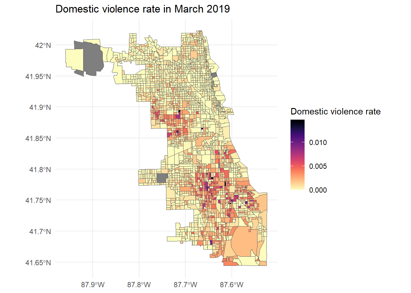
3.2 The Spatial Distribution of Domestic Violence Rate
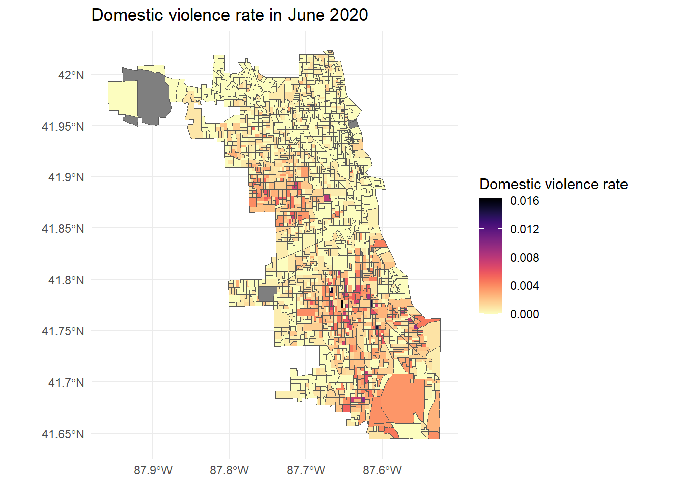
This section visualizes the spatial distribution of domestic violence in the geographic unit, census block group, by month. The maps indicate the domestic violence rate of each census block group which is calculated by the total number of reported domestic violence divided by the population size.
3.2.1 The variation between March to June (2019 and 2020)
2019 year
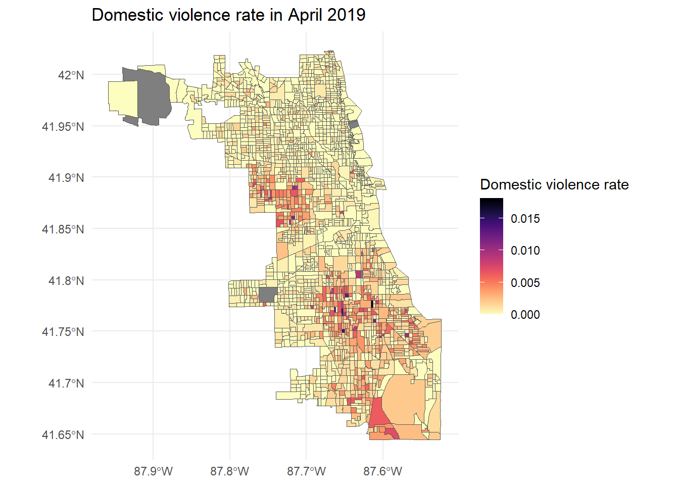
We will first look at the variation of domestic violence between March 2019 to June 2019. Note that the domestic violence rate has been plotted as continuous value and the scales vary between different maps, thus the severity of domestic violence of each month cannot be compared directly. However, there are some significant clustering patterns can be observed from the maps, furthermore, these patterns seem to appear at roughly same locations across different months. It can be implied that there are spatial autocorrelation relationships in the reported domestic violence.
March 2019
April 2019
May 2019

June 2019

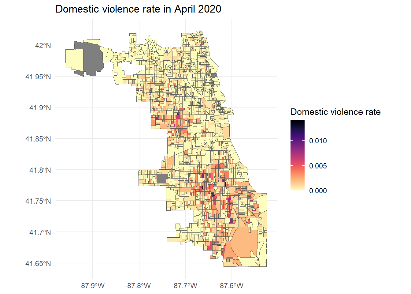
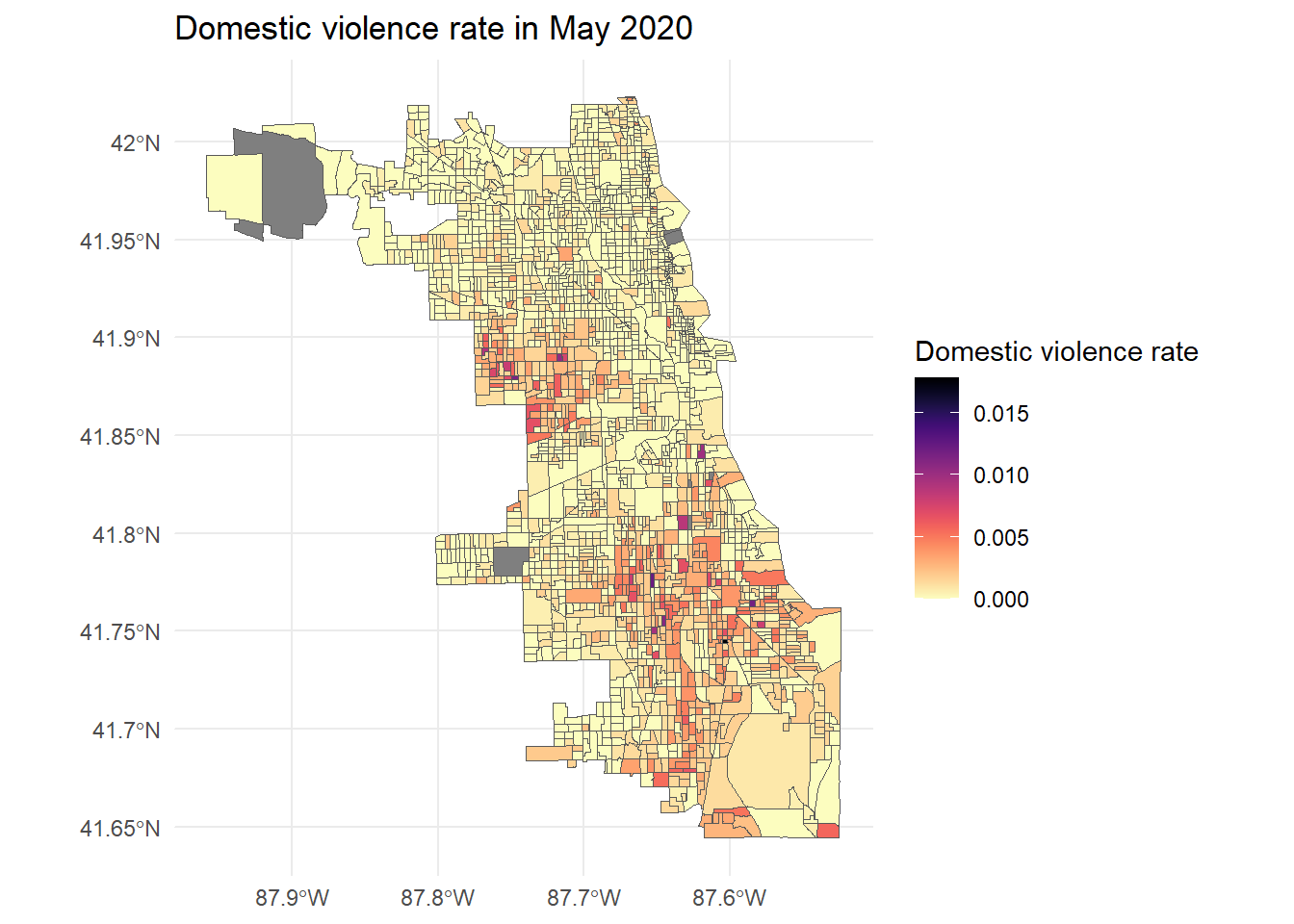
2020 year
Next, We will look at the variation of domestic violence between March 2020 to June 2020. It seems that there are fewer census block groups have reported domestic violence in March 2020 and April 2020 (More census block groups are colored as light-yellow). There are still some significant clustering patterns across each month.
March 2020

April 2020
May 2020
June 2020
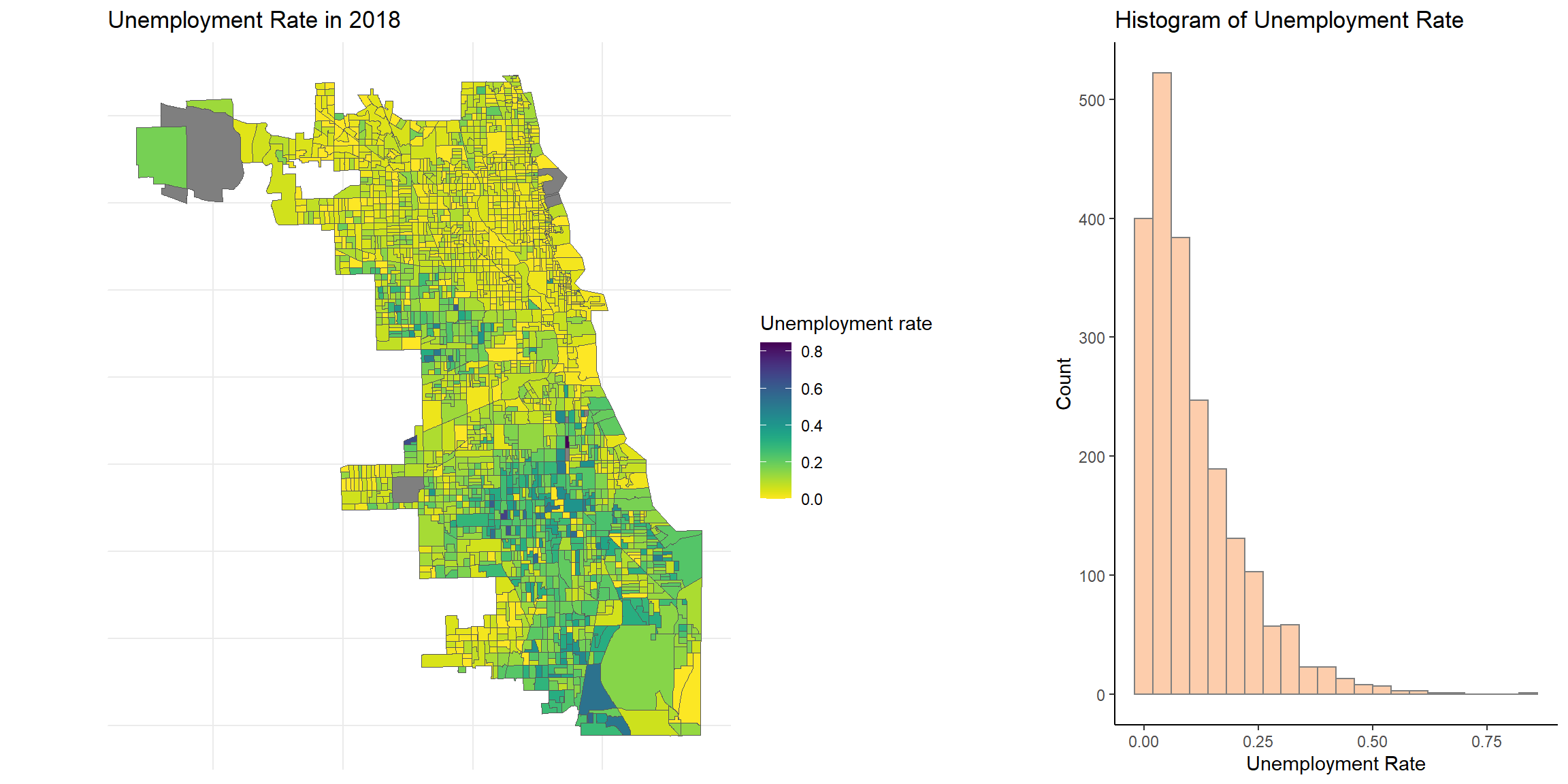
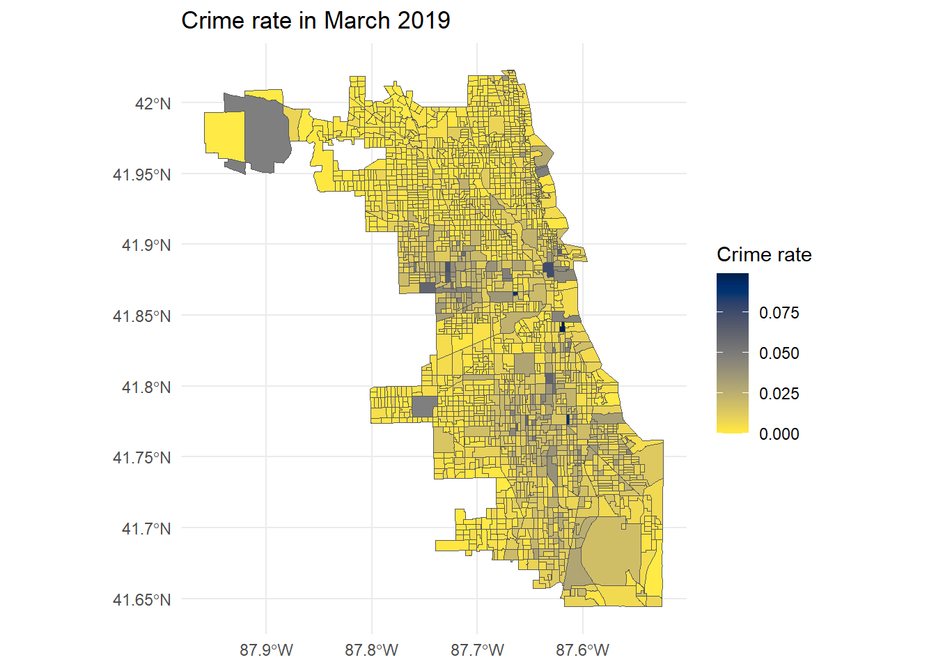
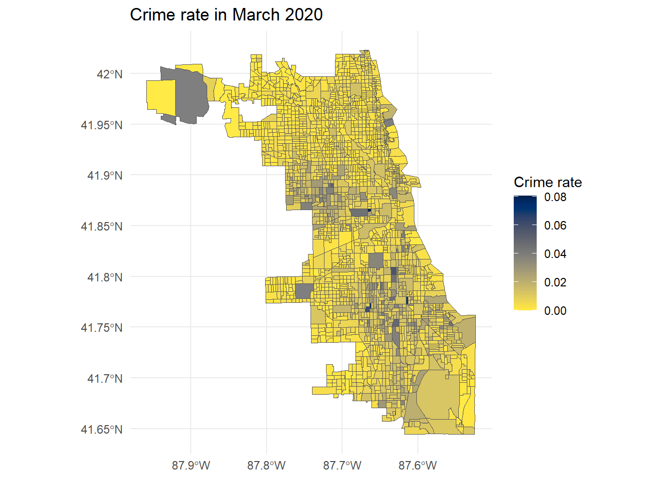
3.3 The Spatial Distribution of Socio-economic Indicators
Finally, let’s explore the spatial distribution of several socio-economics indicators that have been found to be related to domestic violence (Beyer, Wallis & Hamberger, (2013)). The spatial patterns of these indicators can be compared with the spatial distribution of domestic violence. It can be observed that: 1. The areas with lower median household income have higher domestic violence rate; 2. The areas with higher unemployment rate have higher domestic violence rate; 3. The areas with higher crime rate also show higher domestic violence rate.
Median household income

Unemployment rate
Crime rate
March 2019
April 2019

March 2020
April 2020

4 Conclusions
There are few points could be concluded from the above analysis:
Despite several countries have reported higher domestic violence after the lock-down policy has imposed (Ertan et al., (2020); Bradbury‐Jones and Isham, (2020)), the reported domestic violence in Chicago City has actually decreased.
The domestic violence rate maps imply that there might be spatial autocorrelation relations in the reported domestic violence. It also validates the above point that there are fewer census block groups have reported domestic violence in March 2020 and April 2020.
The spatial distributions of the selected socio-economic indicators are highly associated with the distribution of domestic violence rate.
One possible reason the domestic violence has decreased after the lock-down could be that it might be more difficult for the victims to reach out for help when they were constrained at home with the main abusers. Another reason could be that using crime reported data as data source suffers from a main issue, crime tends to be under-reporting. In particular, domestic violence crime has been considered as one of the most under-reporting crime type.
For the future direction of this project, I think it is crucial to look at the reasons of why reported domestic violence have decreased dramatically and to examine whether the domestic violence is under-reporting. The associations between socio-economic indicators and domestic violence might be a good starting point, if we could find more predictors for domestic violence, it might be possible to predict the domestic violence during lock-down time period. As as result, the predicted domestic violence could be compared with the reported domestic violence, and the results might give us some clues.
5 References
Beyer, K., Wallis, A. B., Hamberger, L. K. (2013), Neighborhood environment and intimate partner violence: a systematic review. Trauma, Violence, & Abuse, 16(1):16-47. https://doi.org/10.1177/1524838013515758
Bradbury‐Jones, C. and Isham, L. (2020), The pandemic paradox: The consequences of COVID‐19 on domestic violence. Journal of Clinical Nursing, (29): 2047-2049. https://doi.org/10.1111/jocn.15296
Ertan, D., El-Hage, W., Thierree, S., Javelot, H., and Hingray, C. (2020), COVID-19: urgency for distancing from domestic violence. European Journal of Psychotraumatology, (11), 18800245. https://doi.org/10.1080/20008198.2020.1800245