GEO 511 Final Project
Housing Violations by Neighborhood
Brendan Kunz
Introduction
[~ 200 words]
Clearly stated background and questions / hypotheses / problems being addressed. Sets up the analysis in an interesting and compelling way.
For my project, I’ll be looking at 311 requests in Buffalo that allege code violations by landlords, stretching from 2008 to the beginning of 2020. This issue caught my interest because in a previous internship during my undergrad, I would canvass in mostly low income neighborhoods of Binghamton where I was able to see the negligence of slum lords in these areas. Within Binghamton, these poor living conditions for renters was mostly confined to a handful of neighborhoods so I’m wondering if I will be able to see something similar in Buffalo by looking at the 311 requests. Also I’m interested in looking at a number of demographics that might correspond with high housing violations such as the tendency for racial minorities to be confined largely to low-income, underdeveloped neighborhoods and also poverty rates. Going into this, it’s important to note that issues concerning housing are highly complex and no single factor is going to be able to explain this and the data provided doesn’t account for what percent of housing units are rentals and what the density of the neighborhoods are to begin with.
Materials and methods
[~ 200 words]
See http://rmarkdown.rstudio.com/ for all the amazing things you can do.
Load any required packages in a code chunk (you may need to install some packages):
library(tibble)
library(rgdal)
library(sp)
library(sf)
library(GISTools)
library(RColorBrewer)
library(tbart)
library(viridis)
library(dplyr)
require(rgdal)
library(ggmap)
library(ggplot2)
library(raster)
library(tmap)
library(kableExtra)
knitr::opts_chunk$set(cache=TRUE)  # cache the results for quick compiling
Download and clean all required data
All of the data downloaded and referenced in this project is either from the 311 requests data found in OpenDataBuffalo or from the neighborhood profile data lens which can also be found from OpenDataBuffalo.
#neighborhoods <- st_read(dsn = path.expand("violation_count2.shp"), layer = "violation_count2")
URL <- "https://raw.githubusercontent.com/geo511-2020/geo511-2020-project-btkunz/master/violation_count3.geojson"
neighborhoods <- st_read(dsn = URL)
## Reading layer `violation_count3' from data source `https://raw.githubusercontent.com/geo511-2020/geo511-2020-project-btkunz/master/violation_count3.geojson' using driver `GeoJSON'
## Simple feature collection with 35 features and 14 fields
## geometry type: MULTIPOLYGON
## dimension: XY
## bbox: xmin: -78.91246 ymin: 42.82603 xmax: -78.79504 ymax: 42.96641
## geographic CRS: WGS 84#neighborhood <- st_as_sf(neighborhoods,4326)library(tmap)
library(ggmap)
#Expand bbox to accommodate for a title and legend
nbhd_bbox <- st_bbox(neighborhood)
xrange <- nbhd_bbox$xmax - nbhd_bbox$xmin
yrange <- nbhd_bbox$ymax - nbhd_bbox$ymin
nbhd_bbox[1] <- nbhd_bbox[1] - (0.3 * xrange) #learned how to efficiently adjust the bbox from stack overflow
nbhd_bbox[3] <- nbhd_bbox[3] + (0.3 * xrange)
nbhd_bbox[2] <- nbhd_bbox[2] - (0.2 * yrange)
nbhd_bbox[4] <- nbhd_bbox[4] + (0.2 * yrange)URL2 <- "https://raw.githubusercontent.com/geo511-2020/geo511-2020-project-btkunz/master/Neighborhood_Statistics.geojson"
demographics <- st_read(dsn = URL2)## Reading layer `Neighborhood_Statistics' from data source `https://raw.githubusercontent.com/geo511-2020/geo511-2020-project-btkunz/master/Neighborhood_Statistics.geojson' using driver `GeoJSON'
## Simple feature collection with 35 features and 135 fields
## geometry type: MULTIPOLYGON
## dimension: XY
## bbox: xmin: -78.91246 ymin: 42.82603 xmax: -78.79504 ymax: 42.96641
## geographic CRS: WGS 84#st_as_sf(demographics,4326)
#Edits to the bbox to accommodate for a title and legend
buff_bbox <- st_bbox(demographics)
print(buff_bbox)## xmin ymin xmax ymax
## -78.91246 42.82603 -78.79504 42.96641xrange <- buff_bbox$xmax - buff_bbox$xmin
yrange <- buff_bbox$ymax - buff_bbox$ymin
buff_bbox[1] <- buff_bbox[1] - (0.25 * xrange) #learned how to efficiently adjust the bbox from stack overflow
buff_bbox[3] <- buff_bbox[3] + (0.25 * xrange)
buff_bbox[2] <- buff_bbox[2] - (0.2 * yrange)
buff_bbox[4] <- buff_bbox[4] + (0.2 * yrange)Add any additional processing steps here.
Results
[~200 words]
Tables and figures (maps and other graphics) are carefully planned to convey the results of your analysis. Intense exploration and evidence of many trials and failures. The author looked at the data in many different ways before coming to the final presentation of the data.
Show tables, plots, etc. and describe them.
Housing Violations Map
tm_shape(neighborhood, bbox = nbhd_bbox)+
    #tm_polygons(col = "NUMPOINTS", palette = blues9)+
    tm_fill("NUMPOINTS", title = "Housing\nViolations", palette = blues9, n = 9)+
    tm_borders()+               #helped by Collin
    tm_layout(title = "Housing Violations By Neighborhood", title.position = c("center","top"),
              title.bg.color = "gray", title.bg.alpha = 0.5)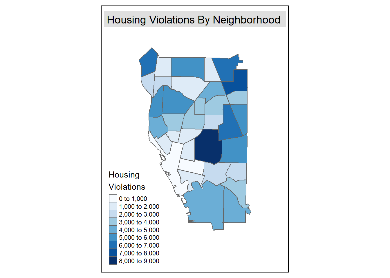
With this map, what I found to be informative is how the housing violations seem to be clustered largely in the East side, around UB South campus, and isolated sections of the West side. While I expected the number to be high in the East side and parts of the West side due to the poor state of the housing stock in that area, I was a bit surprised at the higher concentration in the upper bounds of the West side, as I never viewed that area as having issues with housing quality.That being said, the distribution of violations by neighborhood won’t be perfectly representative of the actual situation because different neighborhoods have various percentages of units that are rentals and might be less populous due to an abundance of vacant lots.
Poverty Rate Map
tm_shape(demographics, bbox = buff_bbox)+
   tm_fill("Poverty.Ra", title = "Poverty Rate", palette = blues9, n = 9)+
   tm_borders()+
   tm_layout(title = "Poverty Rate By Neighborhood ", title.position = c("center","top"), title.bg.color = "gray",
             title.bg.alpha = 0.5)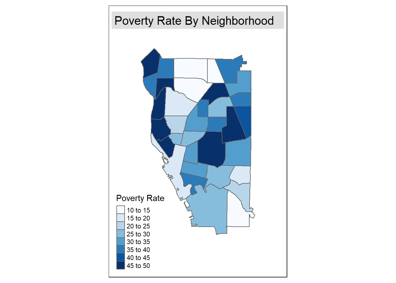
This map focuses on the issue of economic segregation in Buffalo that many of us are already aware of, where North and South Buffalo are predominately middle class while the East side and parts of the West side are predominately lower income. As stated above, my initial thoughts were that violation reports would be largely concentrated in the East and West sides of Buffalo due to what I perceived to be a large number of rentals relative to the other areas of the city.
Racial Demographics Map
tm_shape(demographics, bbox = buff_bbox)+
   tm_fill("Percent.Wh", title = "Percent\nWhite", palette = blues9, n = 9)+
   tm_borders()+
   tm_layout(title = "Percent White By Neighborhood", title.position = c("center","top"), title.bg.color = "gray",
             title.bg.alpha = 0.5)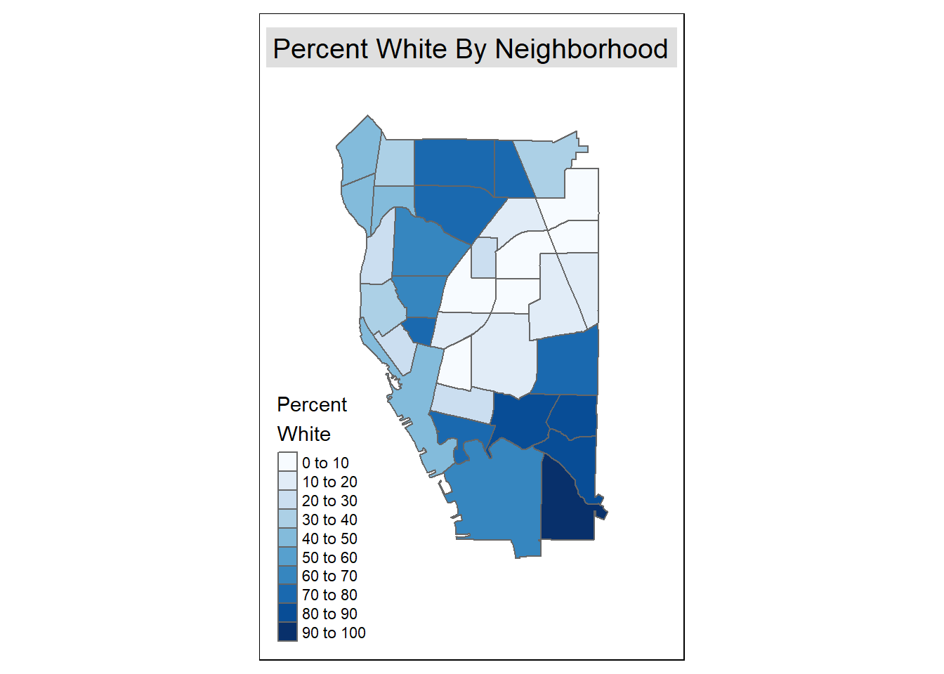
I set this neighborhood to percent white as unfortunately, OpenDataBuffalo doesn’t have a field for all nonwhite racial groups. What this graph shows us when compared to housing violations is that there is a strong correlation between issues of rentals being poorly maintained by the owners and these rentals being in majority-minority neighborhoods. That being said, it’s important to take this finding with a grain of salt, as while there is a correlation, the true strength of this correlation is difficult to verify as there can be other issues behind the scenes such as whether the housing violation calls were deemed to be justified or not and how some neighborhoods are dominated by single family homes that are largely owned by their occupants.
#Rental Sharers Map
tm_shape(demographics, bbox = buff_bbox)+
   tm_fill("Share.Rent", title = "Percent\nShare\nRent", palette = blues9, n = 9)+
   tm_borders()+
   tm_layout(title = "Percent Rent Sharers By Neighborhood", title.position = c("center","top"), title.bg.color = "gray",
             title.bg.alpha = 0.5)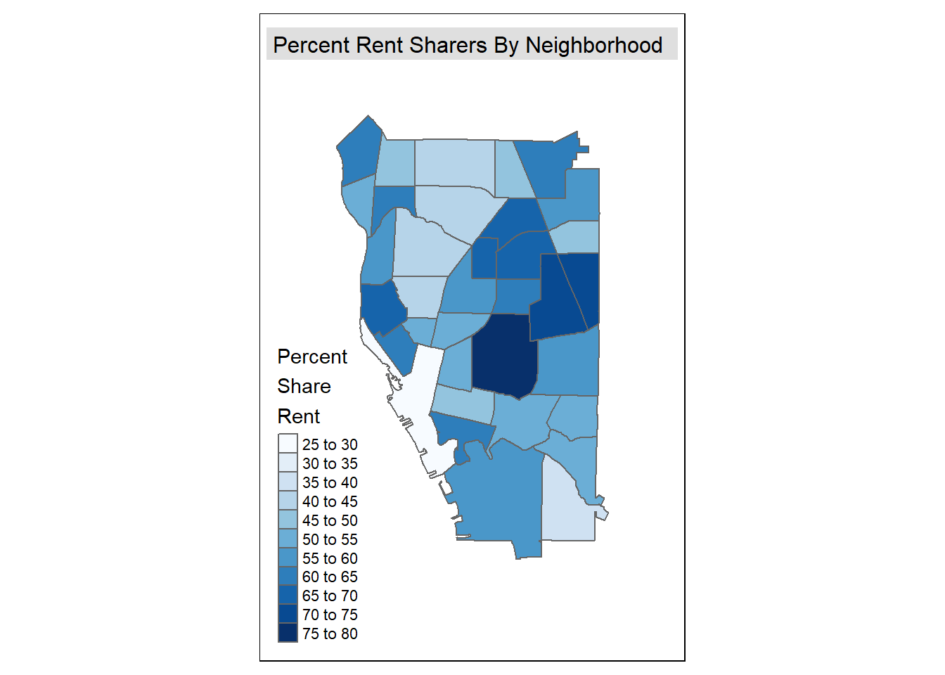
This map seems to give us a fairly clear correlation between having apartment rent split between roommates and higher levels of housing violations. This could potentially be linked back to the issue of poverty where some people who don’t have enough money must live with roommates in lower income areas of cities that they can afford. There is a chance that some units may have an overcrowding issue caused by problematic landlords that are reluctant to make necessary repairs to the properties they own, so that could be something to look into more if I can find more detailed data outside of OpenDataBuffalo.
Conclusions
[~200 words]
Clear summary adequately describing the results and putting them in context. Discussion of further questions and ways to continue investigation.
After finishing all of the maps that I’m using to gather information on what seems to correlate to higher numbers of housing violations, it seems that housing violations are fairly representative of the issues of racial and economic segregation that is seen in Buffalo. As seen in the maps displayed above, the highest concentration of housing violations comes from the Broadway-Fillmore neighborhood within the East Side. As I lack a lot of knowledge of that neighborhood, I believe it would be interesting to look at potential reasons as to why the number of housing violations in this neighborhood is so far above other neighborhoods with otherwise similar demographics. From what information I’ve been able to gather it seems that areas where people tend to share an apartment and split rent with others have a higher prevalence of housing violations, as can especially be seen in the Broadway-Fillmore neighborhood. Although this project has been a bit inconclusive, the maps corroborate a statement made at the introduction where issues such as poor housing quality are the result of a great many issues rather than just one as I initially felt it possibly could be.
References
All sources are cited in a consistent manner
https://www.jla-data.net/eng/adjusting-bounding-box-of-a-tmap-map/
https://spatialanalysis.github.io/lab_tutorials/4_R_Mapping.html
https://stackoverflow.com/questions/60892033/how-do-you-position-the-title-and-legend-in-tmap
https://www.qgistutorials.com/en/docs/performing_spatial_joins.html
https://data.buffalony.gov/view/bfab-gy8p
https://data.buffalony.gov/Quality-of-Life/311-Service-Requests-Opened-in-2018/3m6w-6utv
https://data.buffalony.gov/Economic-Neighborhood-Development/Neighborhoods/q9bk-zu3p